Matlab files discussed in this section:
branch.m, trimtreeplot.m, trimtreelayout.m
Files for downloading:
gzipped tar-archive
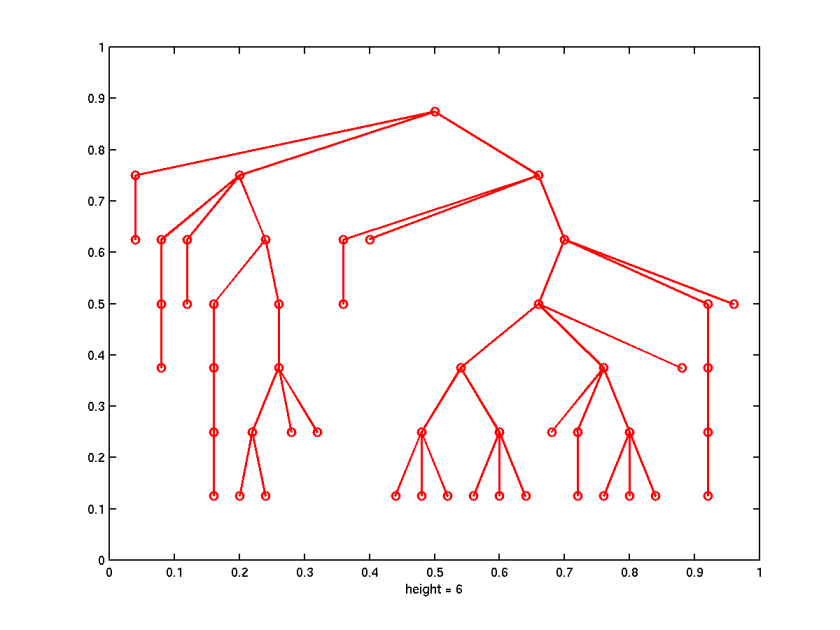
A nice example to illustrate both the MATLAB tools for dealing with tree structures as well as stochastic systems with the Markov property could be a branching or Galton-Watson process. The process describes a population in which each individual gives birth to a random number of children independently of the others and according to the same distribution. The process can be conveniently represented as a random tree. Figure 1 shows the plot of the output of the procedure branch.m from the simulation of the branching process where each individual can have up to 3 children with probabilities [0.2 0.3 0.1 0.4].
 |
In order to implement a branching process, we need to find a suitable implementation for a tree-structure. MATLAB 5 appears to have at least two implementations of trees: one in the Wavelet toolbox and one in the Sparfun toolbox. In the wavelet context trees are used in a slightly unconventional manner, so the version of the tree-structure in the Sparfun toolbox seems to be more optimal for the branching processes.
In the Sparfun toolbox a tree is represented as a vector, the ith element of which is the index number of the parent of the node i. This allows to have any ordering conventions as well as fast reconstruction of the adjacency matrix of the tree. In such a way, the tree in Figure 1 is the vector [0 1 1 1 2 3 4 3 4 3 4 6 7 8 10 10 11 11 11 12 15 16 18 17 17 17 21 23 24 24 22 25 22 25 22 25 27 28 34 31 31 29 30 36 29 30 36 29 30 36].
Such implementation of a tree suggests the following algorithm for the simulation of the branching process. In each generation we generate a random vector with a number of children for each individual and add new nodes to the tree as follows. If the individual with the index number k gives birth to n(k) descendants, we add the number k to the tree-vector n(k) times.
Consider now the code in the procedure branch.m. It contains 2 nested loops:
 for i=1:n_gen
   [...]
   for j=1:max_kids
     [...]
   end
 end
and they seem unavoidable due to the dependency structure of the
process. Even if individuals in each generation produce offspring
independently of each other, the number of descendants depends on the
population size of that generation. This means that we need to cycle along
generations. However, the number of individuals in a certain generation
depends only on the number of individuals in the previous generation
which reflects the Markovian nature of the process.
In the outer loop a new generation in the population is generated according to the last existing generation. We start by finding the index numbers for the parent generation:
par_ind = length(parent)-n_kids+1:length(parent);Only the total number of parents matters for the number of children, which allows us to avoid cycling over all individuals in the parent generation. Indeed, the efficient MATLAB vector commands give the numbers of offspring for all parents at once. To generate a sample vector from the offspring distribution start as usual by generating a sample from the uniform distribution in the interval (0,1):
coin = rand(1, n_parents);A classical and simple method to transform a uniform sample to a sample from a discrete distribution is as follows. Divide the interval (0,1) into intervals with lengths equal to the probabilities for the values of the discrete distribution. As values of the discrete distribution we use the indices of the intervals in which the samples of the uniform distribution fall. This is done in a small loop inside the first one, which cycles up to the maximal possible number of children. In this loop we find which parents give birth to exactly j children according to our uniform sample:
j_ind = par_ind(find((coin>cum_prob(j)) & (coin<=cum_prob(j+1))));The command says "find indices of those values in the uniform sample that fall into the interval (p(j), p(j+1)] and select the corresponding indices in the parent generation". It remains to add the indices of parents obtained in this way to the tree-vector, each index replicated j times:
parent = [parent repmat(j_ind, 1, j)];This makes numbering of the nodes in the tree somewhat random, but this does not matter in our context.
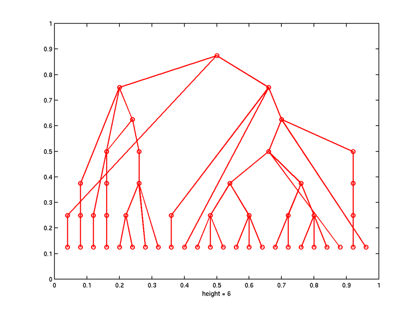
To our disappointment, we found that the standard command TREEPLOT in
the Sparfun toolbox is not suited to plot a tree representing
the branching process. TREEPLOT plots the leaves (the nodes without
offspring) in the deepest layer of the tree, so that the tree in
Figure 1 would appear as follows (TREEPLOT v.6 used):
 |